As mentioned in previous sections, the vanilla perceptron, while
simple and beautiful, suffers from many problems:
it does not converge with inseparable data
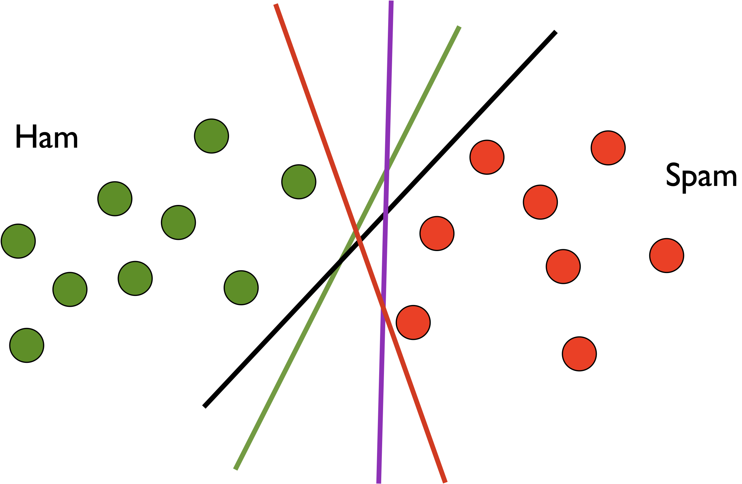
it does not optimize the margin for separable data (as we
discussed in the convergence and proof, if the data is separable, there
are infinitely many weight vectors that separates the data, and
perceptron just returns an arbitrary one of them). Clearly, we would
prefer a “large margin” weight vector which should generalize better on
the unseen test data:
its output weight vector is sensitive to the order of examples,
and later updates dominates earlier ones
As a result, with the publication of the Minksy and
Papert (1969) book on Perceptrons pointing out all these problems,
research on perceptron was dead for 30 years, until Freund and Schapire
revived it in their breakthrough
paper in 1999 where they proposed two simple variations of
perceptron: the voted perceptron and the averaged perceptron, with two
major improvements:
both of them are more stable than the vanilla perceptron in that
they are much less sensitive to the order of examples
both of them output “large margin” weight vectors instead of an
arbitrary one (though not necessarily the “maximum margin” vector)
Between the two versions, the averaged perceptron is much simpler
than voted perceptron, and runs almost as fast as the vanilla
perceptron, but with much better generalization on test data.
Voted Perceptron
The key observation here is that later updates often dominate earlier
ones. This because, as mentioned before, for any mistake on example
\((\vecx, y)\), the new weight vector
after the update, \[ \vecw' \gets \vecw +
y\vecx \] is always better on this example than the old vector
\(\vecw\), though not necessarily
correcting the mistake. More specifically, the new dot product \[ \vecw'\cdot \vecx = \vecw \cdot \vecx +
y\vecx^2 \] is always larger than the old dot product for
positive examples and less than the old one for negative examples.
However, this update might introduce mistakes on previously correct
examples. Therefore, the vanilla perceptron is sensitive to the order of
examples, and the last few updates would have more influence on the
final result.
How would we alleviate this issue?
The first idea is to record the weight vector after each example in
training data \(D\) (not just after
each update, i.e., you would also record the weight vector even if there
is no update), and then at the end of \(T\) epochs over the whole data, you would
have collected a total of \(T|D|\)
models. At testing time, the voted perceptron simply lets all these
models take a vote, and follows the majority.
The above scheme would need to store all \(T|D|\) models, which would cost \(O(T|D|d)\) space where \(d\) is the feature dimensionality. That is
too inefficient. Note that most of those weight vectors are duplicate:
for example, if there are no updates in a row for 10 consecutive
examples, then all those weight vectors are the same. As perceptron
training progresses, the number of mistakes (or updates) decreases, and
more and more weight vectors will be the same near the end. So can we do
better?
A more efficient way of implementing the voted perceptron is to only
the weight vectors after each update rather than after each
example, and also record the number of votes for each weight
vector (the previous scheme had 1 vote per weight vector). If there is
no update on one example, we just increase the vote of that
weight vector, so that this is equivalent to the original scheme. Now
instead of \(O(T|D|d)\) space you only
need \(O(Ud)\) where \(U\ll T|D|\) is the number of updates.
Freund and Schapire (1999) showed that voted perceptron outputs a
large-margin classifier (though not necessarily the one with
maximum-margin – that would need support vector machines, or SVMs).
Geometrically, for a separable data set, there are infinitely many
weight vectors (or models, or classifiers) that separates the positive
and negative examples, but each model has a different margin. Clearly a
larger margin model will generalize better at testing time. The other
advantage of voted perceptron is stability: because it does not rely on
a single model (the last weight vector) as in vanilla perceptron, and
all intermediate models can vote, it is much more stable and insensitive
to the order of examples.
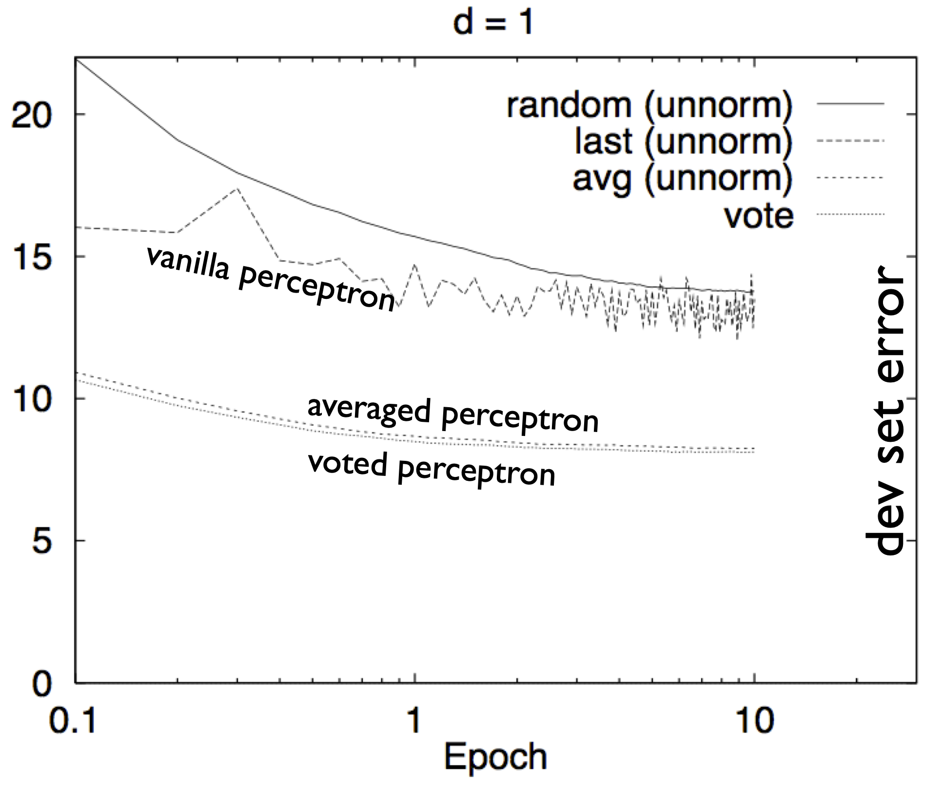
error rates of voted and averaged
perceptrons, from Freund and Schapire 1999
The above figure from their paper showed that vanilla perceptron is
unstable (due to sensitivity to the order of examples), while voted
perceptron is much more stable and generalizes much better on the unseen
dev set (the dev error is lower).
Averaged Perceptron
The voted perceptron is much better than vanilla perceptron, but it
is not very practical. This is because you still have to store
each updated model, needing \(O(Ud)\)
space where \(U\) is the number of
updates. This may not be feasible when you have a high dimensional model
and a big data set. Can we approximate voted perceptron with much less
space? In that same paper, Freund and Schapire also proposed the
averaged perceptron, which is a practical approximation of
voted perceptron that works equally well (in terms of accuracy) with the
former.
Instead of letting each intermediate model vote for the final result,
the new idea is to output the average model, i.e., the average
over all weight vectors after each example (again, not after each
update). However, now you only need to store one extra model,
the running sum over all intermediate models, i.e., \[\vecws \gets \vecws + \vecwi\] after the
\(i\)th example. So at the end, the sum
is \[\vecws = \sum_{i=1}^{T|D|}
\vecwi\] which is your output (note that you do not even need to
normalize it by \(T|D|\) because it
does not change the direction of the vector).
Now we solved the space problem and just need the same \(O(d)\) space as vanilla perceptron. But it
is still not very practical due to time complexity, because you need to
perform this addition to the running sum \(\vecws\) after each example, and in total
this needs \(O(T|D|d)\) time and it is
too slow for high dimensional applications such as natural language. In
those applications, the feature vectors \(\vecx\) are often very sparse (most
dimensions are zeros and only a few are non-zero). The updates are even
sparser because each training example \(\vecx\) (often a sentence) just includes a
dozen or so words, so each update \(\deltaw\) just involves a dozen or so
features. Let us assume
to be the dimensionality of updates (which is the maximum number of
non-zero features, or \(\ell_0\)-norm,
of any example \(\vecx\)).
The vanilla perceptron runs in \(O(U\dupdate)\) time while the naive version
of averaged perceptorn runs in \(O(T|D|d)\) time (\(U \ll T|D|)\) and \(\dupdate \ll d\)).
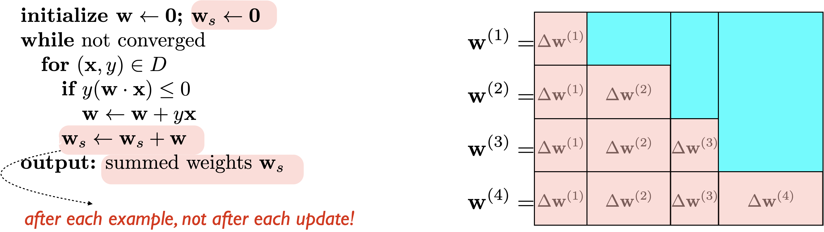
The pseudocode and visualization are shown below:
Efficient
Implementation of Averaged Perceptron
How could we improve the scalability?
Well, the first idea is identical to the idea in improved voted
perceptron: instead of summing the weight vector after each example, we
can save the weight vector after each update, and keep track of each
weight vector’s “vote”. At the end just output a weighted sum \(\vecws = \sum_{i=1}^U \vecwi \cdot v_i\).
This method costs more space (\(O(Ud)\)) but saves time (\(O(Ud)\)), which has identical time and
space complexities with the improved voted perceptron, so still not
practical.
The next key idea is the take advantage of the sparsity in updates.
Since each update is extremely sparse \(\dupdate \ll d\), we should just store the
update vectors\(\deltawi\)
instead of \(\vecwi\). But notice that
each update vector has influence all the way till the end of the
training, so you need to keep track of the influence of each update
vector. For example, assume there are four updates, one on each
example:
This would improve the space to \(O(d+U\dupdate)\) and time to \(O(U\dupdate)\), which is huge improvement,
but still not the best we can do yet.
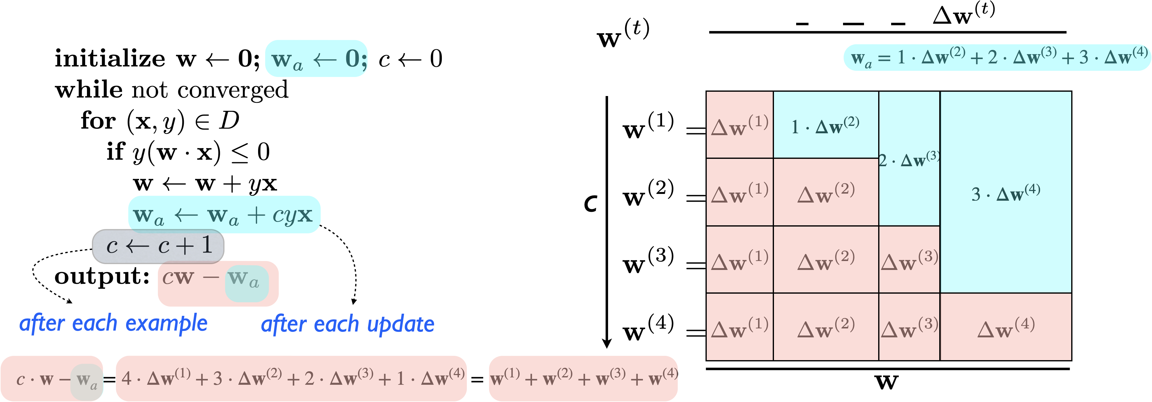
Following this line of thought, Hal
Daumé (2006, PhD thesis) invented a much simpler (and even more
scalable) trick that brings the space and time down to the original
vanilla perceptron. Basically, you just need an auxiliary vector \(\vecw_a\) and a counter \(c\) to count the number of examples (not
updates) so far. Whenever you make an update (\(\vecw\gets \vecw + \deltaw\) where the
update \(\deltaw = y\vecx\)), you would
also update the auxiliary vector
\[\vecw_a\gets \vecw_a +
c\deltaw\]
We can show that in each step, we have the running sum \(\vecws = c\vecw - \vecw_a\). The intuition
is that earlier updates have more influence, but in the auxiliary
vector, earlier updates are weighted less:
The new pseudocode and visualization are shown below:
Now we have the fastest averaged perceptron algorithm, which has
identical time and space as the vanilla perceptron: \(O(d)\) space and \((U\dupdate +d)\) time. The following table
summarizes the complexities of various algorithms.