\(\renewcommand{\vec}[1]{\mathbf{#1}}\)
\(\newcommand{\vecw}{\vec{w}}\) \(\newcommand{\vecx}{\vec{x}}\) \(\newcommand{\vecu}{\vec{u}}\) \(\newcommand{\veca}{\vec{a}}\) \(\newcommand{\vecb}{\vec{b}}\)
\(\newcommand{\vecwi}{\vecw^{(i)}}\) \(\newcommand{\vecwip}{\vecw^{(i+1)}}\) \(\newcommand{\vecwim}{\vecw^{(i-1)}}\) \(\newcommand{\norm}[1]{\lVert #1 \rVert}\)
Under what condition can you tell if the perceptron algorithm will converge on a data set? It turns out that convergence depends on a crucial property of the training data called linear separation. Under that condition, we can rigorously prove that the perceptron has to converge in finite number of steps. This theorem, known as the Perceptron Convergence Theorem, is one of the most important theoretical foundations of machine learning, and its geometric proof is one of the most beautiful proofs in machine learning. The proof technique is used in many other theorems involving online learning.
While the perceptron algorithm was invented by Rosenblatt, this theorem and its proof were from NYU mathematician Albert B. J. Novikoff in 1962 (he is still living as of this writing in 2023!).
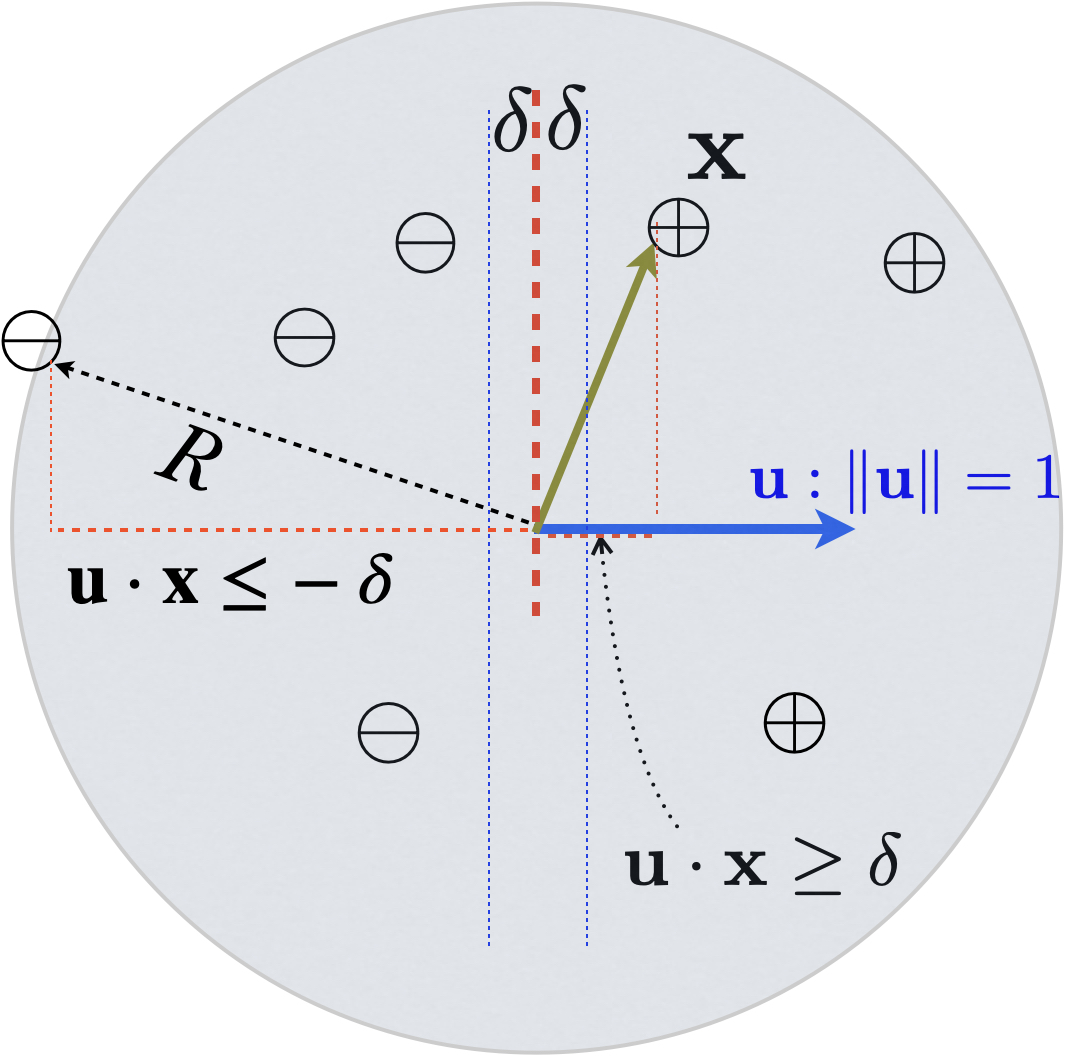
A dataset \(D\) is said to be “linearly separable” if there exists some unit oracle vector \(\vecu: \norm{\vecu}=1\) which correctly classifies every example \((\vecx, y)\) with a margin of at least \(\delta>0\):
\[ y(\vecu\cdot\vecx) \geq \delta, \text{for all } (\vecx, y) \in D \]
Geomtrically, this means the positive and negative examples are separated by a linear buffer zone of at least \(2\delta\) in width. Or in other words, all positive examples are distributed at least \(\delta\) away from the decision boundary (separating hyperplane) \(\vecu\cdot\vecx = 0\), and in the direction of \(\vecu\) (i.e., \(\vecu\cdot\vecx \geq \delta\)), while all negative examples are distributed at least \(\delta\) away from the decision boundary (separating hyperplane) \(\vecu\cdot\vecx = 0\), and in the direction of \(-\vecu\) (i.e., \(\vecu\cdot\vecx \leq - \delta\)).
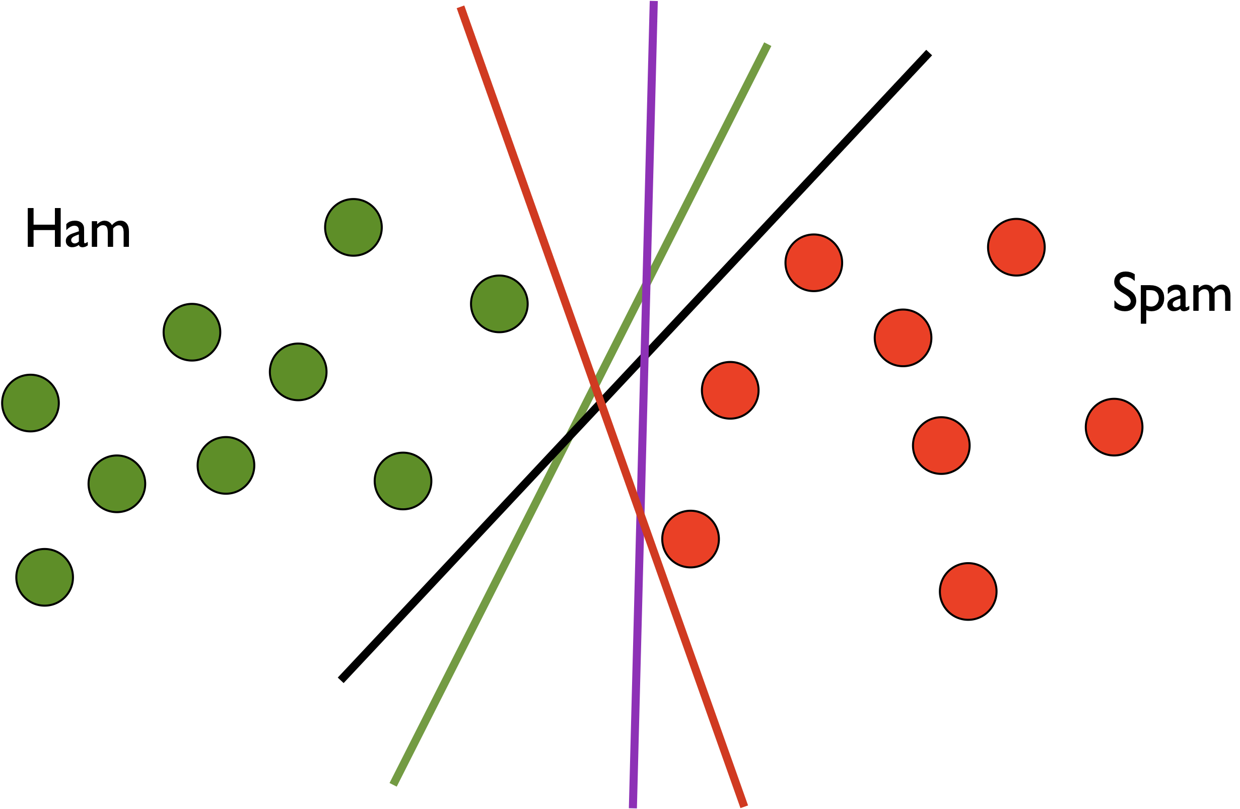
It is important to note that, if a data set is linearly separable, then there exists infinitely many separating hyperplanes (each with a different margin). Each such hyperplane corresponds to one unit oracle vector. The point of the convergence theorem below is that as long as one oracle vector exists (thus infinitely many exist), then the perceptron is bound to find such a vector (and find it fast), but not necessarily the same oracle vector that you have in your mind.
If the training set \(D\) is linearly separable with margin \(\delta\), then the perceptron algorithm (with initial weight \(\mathbf{0}\)) must converge to a linear separator after at most \[\frac{R^2}{\delta^2}\]
mistakes (updates) where \(R= \max_{(\vecx, y) \in D} \norm{\vecx}\) is the “radius” (maximum norm) of the dataset.
This theorem is remarkable in the following aspects regarding the convergence rate \(R^2/ \delta^2\):
The proof of this remarkable convergence proof is also truly remarkable.
The high-level idea of the proof is to bound the weight vector from both above and below. On the one hand, after each update, the weight vector is making some positive progress on the (unknown) oracle direction because such an oracle vector \(\vecu\) does exist due to linear separation; in other words, the weight vector is more and more aligned with the (unknown) oracle vector \(\vecu\). On the other hand, in each update, the increase in the norm of the weight vector is also bounded by the radius \(R\) because each update involves a mistake which implies \[y (\vecw\cdot \vecx) < 0.\]
We can then derive bounds of the norm of \(\vecw\) from both sides, from which we can prove a bound on the number of updates.
First, we know the initial weight vector is \(\vecw^{(0)} = \mathbf{0}\). Let us denote \(\vecwi\) as the weight vector after \(i\) updates (i.e., \(\vecw^{(1)}\) is the one after the first update). Assume the \(i\)th update is on example \((\vecx, y)\), we have:
\[ \begin{align} \vecwi & = \vecwim + y\vecx \\ \vecu\cdot\vecwi & = \vecu\cdot\vecwim + \color{blue} {y(\vecu\cdot\vecx)} & \text{dot product both sides with (unknown) oracle} \\ & \geq \vecu\cdot\vecwim + \color{blue} {\delta} & \text{linear separation: } \forall (\vecx, y)\in D, y(\vecu\cdot\vecx)\geq \delta \\ & \geq i\delta & \text{by induction} \end{align} \]
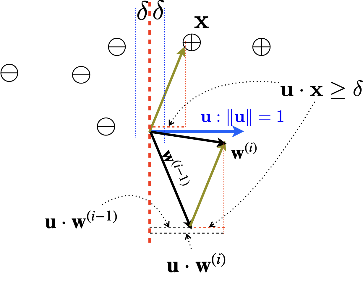
Geometrically, dot product both sides with \(\vecu\) means taking the projection onto the (unknown) oracle direction for both sides, and by the definition of linear separation, \(y\vecx\) must have at least a (positiive) projection length of \(\delta\) on the oracle direction. This means after each update, the projection of weight vector \(\vecw\) on the (unknown) oracle direction \(\vecu\) increases, by at least the margin \(\delta\), which means there is more agreement with the oracle direction. In other words, we are making steady progress in each update towards a correct direction that can separate the positive and negative examples.
After \(i\) updates, the weight vector has at least a positive projection length of \(i\delta\) on the correct direction, i.e., \(\vecu\cdot\vecwi \geq i\delta\). This implies that the norm of \(\vecwi\) is also at least \(i\delta\), since any vector’s norm is at least its projection length on any direction, i.e., \[\norm{\vecwi} \geq \norm{\vecwi} \cos \theta = \vecwi \cdot \vecu \geq i\delta\] where \(\theta\) is the angle between \(\vecw\) and \(\vecu\). Or more formally,
\[\norm{\vecwi} = \norm{\vecu}\norm{\vecwi} \geq \vecu \cdot \vecwi \geq i\delta.\]
In part 1 we achieved a lower bound on the norm of the weight vector after \(i\) updates. Now let us bound it from the above. The intuition is that after each update, the weight vector norm might grow, but not by too much, because there is a bound on the radius (maximum norm of \(\vecx\)), and because the update is on a mistake, thus with a “negative” dot product.
\[ \begin{align} \norm{\vecwi}^2 & = \norm{\vecwim + y\vecx}^2 \\ & = \norm{\vecwim}^2 + \norm{y\vecx}^2 + 2\vecwim \cdot (y\vecx) & \norm{\veca\! +\!\vecb}^2 = (\veca\!+\!\vecb)^2 = \veca^2\!+\!\vecb^2 \!+\! 2\veca\cdot\vecb\\ & = \norm{\vecwim}^2 + \color{red}{\norm{\vecx}^2} + \color{blue}{2y(\vecwim \cdot \vecx)}\\ & \leq \norm{\vecwim}^2 + \; \color{red}{R^2} \;\; + \color{blue}{0} & \text{update on a mistake: $y(\vecwim\cdot\vecx)<0$}\\ & \leq i R^2 &\text{by induction} \end{align} \]
The crucial step is that each update is on a mistake, thus \(y(\vecwim \cdot \vecx)<0\). 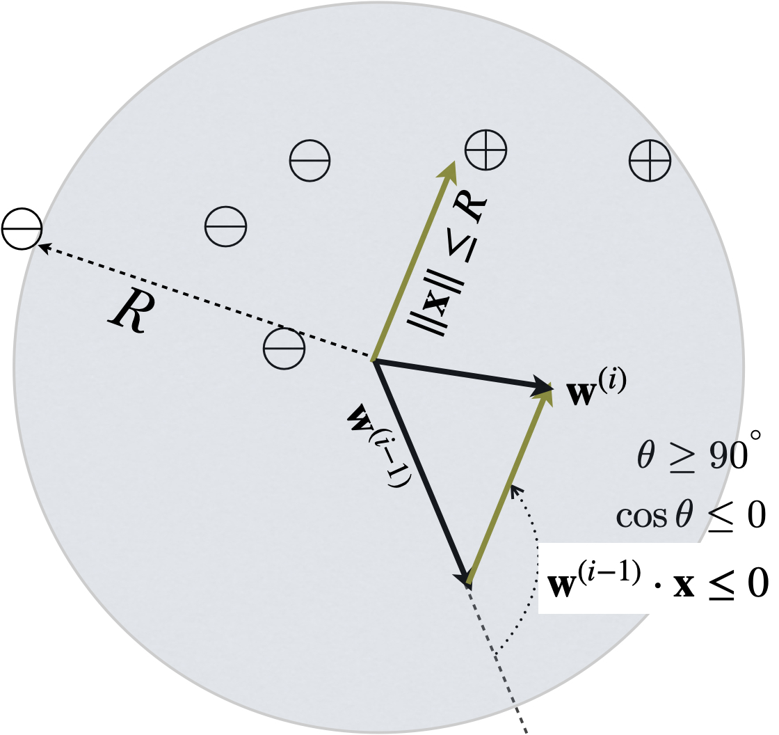
Combining the two bounds, we have:
\[ i^2 \delta^2 \leq \norm{\vecwi}^2 \leq i R^2\] thus the number of updates (or mistakes) is at most \[ i \leq \frac{R^2}{\delta ^2}.\]
This completes the proof.