\(\renewcommand{\vec}[1]{\mathbf{#1}}\)
\(\newcommand{\vecw}{\vec{w}}\) \(\newcommand{\vecx}{\vec{x}}\) \(\newcommand{\vecu}{\vec{u}}\) \(\newcommand{\veca}{\vec{a}}\) \(\newcommand{\vecb}{\vec{b}}\) \(\newcommand{\vecPhi}{\vec{\Phi}}\)
\(\newcommand{\vecwi}{\vecw^{(i)}}\) \(\newcommand{\vecwip}{\vecw^{(i+1)}}\) \(\newcommand{\vecwim}{\vecw^{(i-1)}}\) \(\newcommand{\norm}[1]{\lVert #1 \rVert}\)
The perceptron convergence theorem is very beautiful, but it assumes linear separability of data. In practice, however, data is almost always inseparable, so we need to answer a few questions in this section:
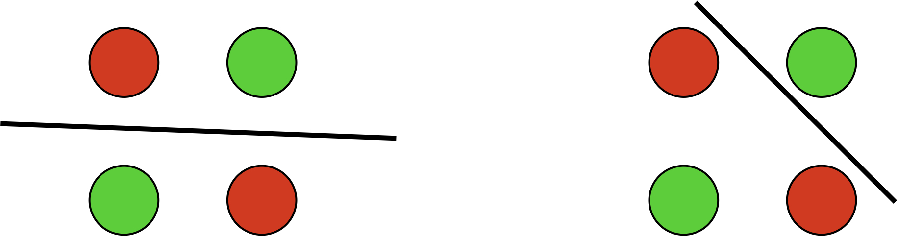
The classical example of the simplest data set that is not linearly separable is the XOR data set:
| \((x_1, x_2)\) | \(y\) |
|---|---|
| \((+1,+1)\) | \(+1\) |
| \((+1,-1)\) | \(-1\) |
| \((-1,-1)\) | \(+1\) |
| \((-1,+1)\) | \(-1\) |
Basically, \(y=x_1 x_2\), which is a nonlinear relation. Note that for simplicity reasons, we did not show the bias dimension in this section, but the augmented space with \(x_0=1\) does not have any impact on the separability on this data set.
This example is obviously not linearly separable, i.e., there does not exist any weight vector that can correctly classify all four examples. Because of this, the perceptron algorithm will not be able to converge either (it will always make mistake(s) on at least one example in each iteration). What is worse, it was shown in the famous book “Perceptrons” (Minsky and Papert, 1969) that finding the minimum error linear separator is NP-hard. This negative result and the pessimistic view around it effectively killed the study of perceptron and neural networks in the 1970s. It was not until the late 1990s that perceptron came back into living, which we will discuss in the next section.
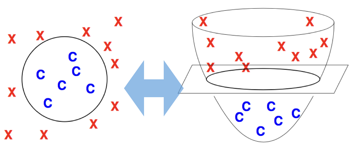
How should we solve the XOR example using a linear classifier? Well, we need some non-linear features, which map the original data into a higher dimensional space. In that space, the data is linearly separable, and we can train our perceptron to get a linear decision boundary. Then we map it back to the original low-dimensional space, and get a non-linear decision boundary.
For example, in the XOR case, we add a quadratic feature \(x_3=x_1 x_2\):
| \((x_1, x_2)\) | \(x_3=x_1 x_2\) | \(y\) |
|---|---|---|
| \((+1,+1)\) | \(+1\) | \(+1\) |
| \((+1,-1)\) | \(-1\) | \(-1\) |
| \((-1,-1)\) | \(+1\) | \(+1\) |
| \((-1,+1)\) | \(-1\) | \(-1\) |
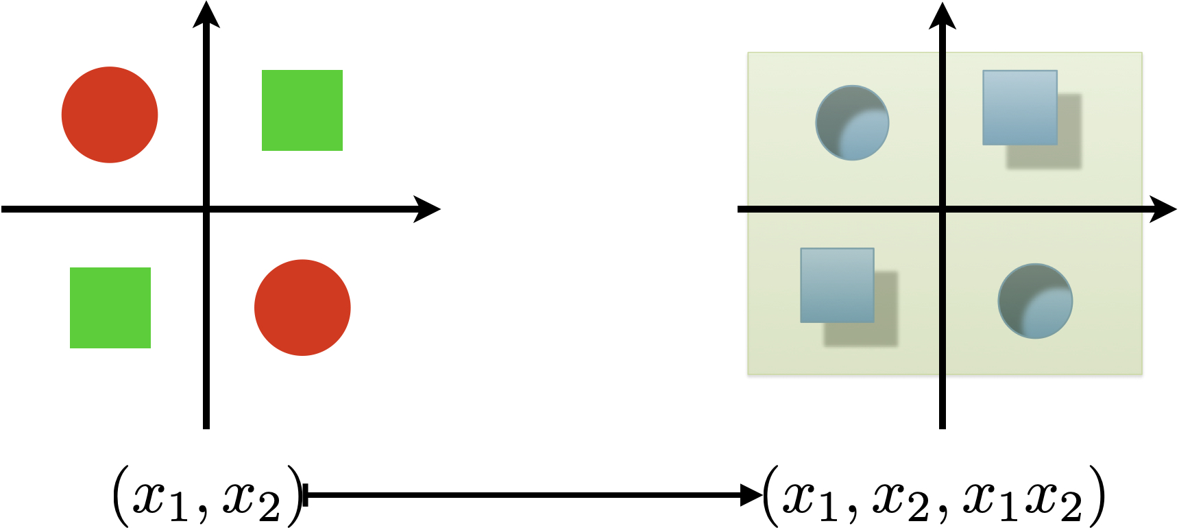
Now in the 3D space, the data is clearly separable, e.g., by the plane \(y=0\). When we map this 3D decision boundary back to 2D, we get a non-linear boundary: quadrants I and III are positive, and quadrants II and IV are negative, which perfectly solves the XOR problem.
In general, you can add many such higher-order “combination” features (\(x_1 x_2\) is a second-order feature), and these are special cases of “polynomial kernels” in kernel methods (which is beyond the scope of this course).
To summarize:
| not linearly separable in low dimensions | \(\stackrel{\text{feature map}}{\Longrightarrow}\) | linearly separable in high dimensions |
|---|---|---|
| \(\Downarrow\) | \(\Downarrow\) | |
| nonlinear decision boundary in low dimensions | \(\stackrel{\text{project back}}{\Longleftarrow}\) | linearly decision boundary in high dimensions |
Now we need to rethink and redefine the notion of separability. As you saw above, technically it is not correct to say that a dataset is separable or not, but rather it is separable under a feature map. In other words, it is the features that make a data set separable. So we redefine:
A dataset \(D\) is said to be “linearly separable” under feature map \(\vecPhi(\cdot)\) if there exists some unit oracle vector \(\vecu: \norm{\vecu}=1\) which correctly classifies every example \((\vecx, y)\) with a margin of at least \(\delta>0\):
\[ y(\vecu\cdot\vecPhi(\vecx)) \geq \delta, \text{for all } (\vecx, y) \in D \]
Now we also restate the perceptron convergence theorem:
If the training set \(D\) is linearly separable under feature map \(\vecPhi\) with margin \(\delta_\vecPhi(D)>0\), then the perceptron algorithm (with initial weight \(\mathbf{0}\)) must converge to a linear separator after at most \[\frac{R_\vecPhi^2(D)}{\delta^2_\vecPhi(D)}\]
mistakes (updates) where \(R_\vecPhi(D)= \max_{(\vecx, y) \in D} \norm{\vecPhi(\vecx)}\) is the “radius” (maximum feature norm) of the dataset.