In classification, you train a machine learning model to classify an input object (could be an image, a sentence, an email, or a person described by a group of features such as age and occupation) into two or more classes. The very basic (and most widely used) setting is “binary classification” where the output label is binary, e.g., whether an image contains a human, whether an email is spam, whether a review is positive or negative, or whether a person (based on his/her features) is likely to earn more than 50K annually. On the other hand, “multiclass classification” classifies an input object into one of the many classes; for example, handwritten digit classification (ten classes, 0-9) is widely used by USPS, and intent classification (need help, complaint, general inqury, etc.) is widely used in dialog systemes deployed in customer service.
The simplest yet still very powerful models in classification is linear classification. What do we mean by “linear classification”? Well, we mean that the model is a linear model, i.e., its decision is based on the linear combination of input features. For example, let us consider a (very crude) toy example: classifying a person based on two features, age (\(a\)) and number of working hours per week (\(t\)), into whether this person is likely to earn 50K or more annually. The intuition is that a person with more experience (age) and more working hours would tend to earn more. Apparently this would not be very accuate at all, but it serves our purpose of illustration. The linear model just looks at a linear combination (i.e., weighted sum) of these two features, and check whether that weighted sum exceeds a threshold (if it does, we output YES otherwise NO):
\[ w_1 \cdot a + w_2 \cdot t > \theta\]
Here weights \(w_1\) and \(w_2\) and the threshold \(\theta\) are the three parameters to be learned from the training data, which contains many example persons, each with an age and a number of hours, plus the label YES/NO. The goal of the machine learning algorithm is to tune or fit these parameters to perform well on the training set. For example, if in a training set, age is much more important than the number of hours, then you would expect the weight \(w_1\) to be higher after training.
We take \(b=-\theta\), which is often called the bias term, and reorganize the above criteria to a more standard form:
\[ w_1 \cdot a + w_2 \cdot t + b > 0\]
For notational convenience and clarity, we often let \(w_0 = b\) so that we can further rewrite it to:
\[ w_1 \cdot a + w_2 \cdot t + w_0 \cdot 1 > 0\]
which can be simplified using dot product:
\[(w_0, w_1, w_2) \cdot (1, a, t) > 0\]
Here we expressed the linear combination as a dot-product between the weight vector \(\mathbf{w}=(w_0, w_1, w_2)\) and the feature vector \(\mathbf{x}=(x_0, x_1, x_2) = (1, a, t)\). Note that each person will always have the first feature being the constant \(x_0=1\) so that we can express the bias term \(b\) as part of the weight vector (\(w_0\)).
More generally, each input object is mapped to a feature vector \((x_1, x_2, \ldots, x_d)\) in a \(d\)-dimensional space, and we always add one more dimension (the bias dimension) up front so that we have \(d+1\) dimensions:
\[ \mathbf{x} = (x_0, x_1, x_2, \ldots, x_d)\]
where \(x_0=1\) for all inputs. This \(d+1\) dimensional space is called the augmented space. The weight vector \(\mathbf{w}\) is similarly augmented to include the extra bias term \(w_0=b\).
\[ \mathbf{w} = (w_0, w_1, w_2, \ldots, w_d)\]
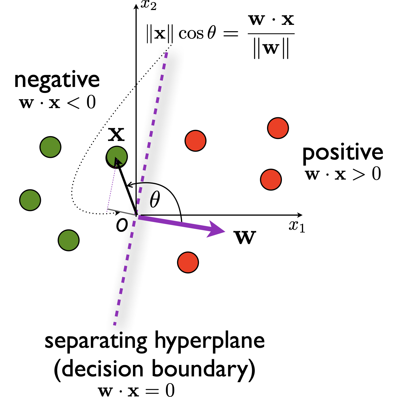
The decision of a linear classifier will now be based on the dot product \(\mathbf{w} \cdot \mathbf{x}\) in the augmented space. If the dot product is positive, i.e.,
\[ \mathbf{w} \cdot \mathbf{x} > 0\]
we output YES, otherwise NO.
Finally, let us define the sign function
\[ \sigma(s) = \begin{cases} 1 & s >0 \\ -1 & \text{otherwise} \end{cases} \]
Now we can express the decision rule of a binary linear classifier as
\[ f(\mathbf{x}) = \sigma(\mathbf{w} \cdot \mathbf{x}) \]
Perceptron is the simplest binary linear classifier and we will see in the next section how to train a perceptron classifier, i.e., how to tune the weights \(\mathbf{w}\) to fit the training data.