Perceptron is the earliest and simplest machine learning algorithm. As disucssed in the last section, we are given a training set \(D = \{(\mathbf{x}^{(i)}, y^{(i)}) \mid i = 1 \ldots |D|\}\) which is a set of training examples \(\mathbf{x}=(1, x_1, \ldots, x_d)\) and their corresponding labels \(y \in \{+1,-1\}\), and want to fit a weight vector \(\mathbf{w}\) so that it can correctly classify all training examples. This means at the end of training, for each training example \((\mathbf{x}, y) \in D\), we would have
\[ \mathbf{w} \cdot \mathbf{x} > 0 \]
If such a weight vector is found during training, we say the perceptron algorithm has “converged”.
It is important to note that as discussed in the last section, we assume the input examples are already in the augmented space, meaning each \(\mathbf{x} = (1, x_1, \ldots, x_d)\) is already in the \(d+1\) dimensional space with one bias feature \(x_0=1\) and \(d\) real features (such as age, gender, number of hours, etc., for a person).
The training procedure of the perceptron algorithm is extremely simple. It could be summarized by the following steps:
initialize weight vector \(\mathbf{w}\)
cycle through the training data (multiple iterations)
until all examples are classified correctly
First, we initialize the weight vector \(\mathbf{w}\) to be the zero vector \(\mathbf{0}\) (in \(d+1\) dimensions), i.e.,
\[\mathbf{w} \gets (0, 0, \ldots, 0)\]
Note that according to the decision rule, this initial weight vector would output negative on all examples since the dot product is always \(0\) and we said we output positive if the dot product is positive and negative if otherwise.
Then we try to improve this weight vector by trial-and-error. Baiscally, we cycle through the training set until convergence (i.e., performing multiple iterations over the whole training data) and make updates to \(\mathbf{w}\). In each iteration, for each training example \((\mathbf{x}, y) \in D\), we try to use the current weight vector to classify it. If the result is different from the correct label \(y\), i.e., the example \(\mathbf{x}\) is positive (\(y=+1\)) but \(\mathbf{w}\cdot \mathbf{x} < 0\) thus outputing negative, or vice versa, we call it a mistake. More formally, a mistake happens when
\[ y \cdot (\mathbf{w}\cdot\mathbf{x}) \leq 0\]
Notice that the tie-breaking case, \(\mathbf{w}\cdot\mathbf{x} = 0\), i.e., when \(\mathbf{x}\) lies exactly on the decision boundary, is also considered a mistake, because we want our model to be strictly correct on each example, not by chance. In other words, the initial zero weight vector would cause a mistake on any training example regardless of the label.
When a mistake happens, we need to improve the weight vector by an update using the mistaken training example. For instance, for a positive example \(\mathbf{x}\) with \(y=+1\), we would hope \(\mathbf{w}\cdot\mathbf{x} > 0\) but the dot product is currently negative or zero. How would we make the dot product more likely to be positive (or at least less negative)? We would add \(\mathbf{x}\) to \(\mathbf{w}\):
\[ \mathbf{w}' \gets \mathbf{w} + \mathbf{x}\]
This way the new dot product is always larger (more positive or less negative) than the original dot product:
\[ \mathbf{w}' \cdot \mathbf{x} = \mathbf{w}\cdot\mathbf{x} + \mathbf{x}\cdot\mathbf{x} > \mathbf{w}\cdot\mathbf{x}\]
because the self dot product \(\mathbf{x}\cdot\mathbf{x} = |\mathbf{x}|^2\) is always positive.
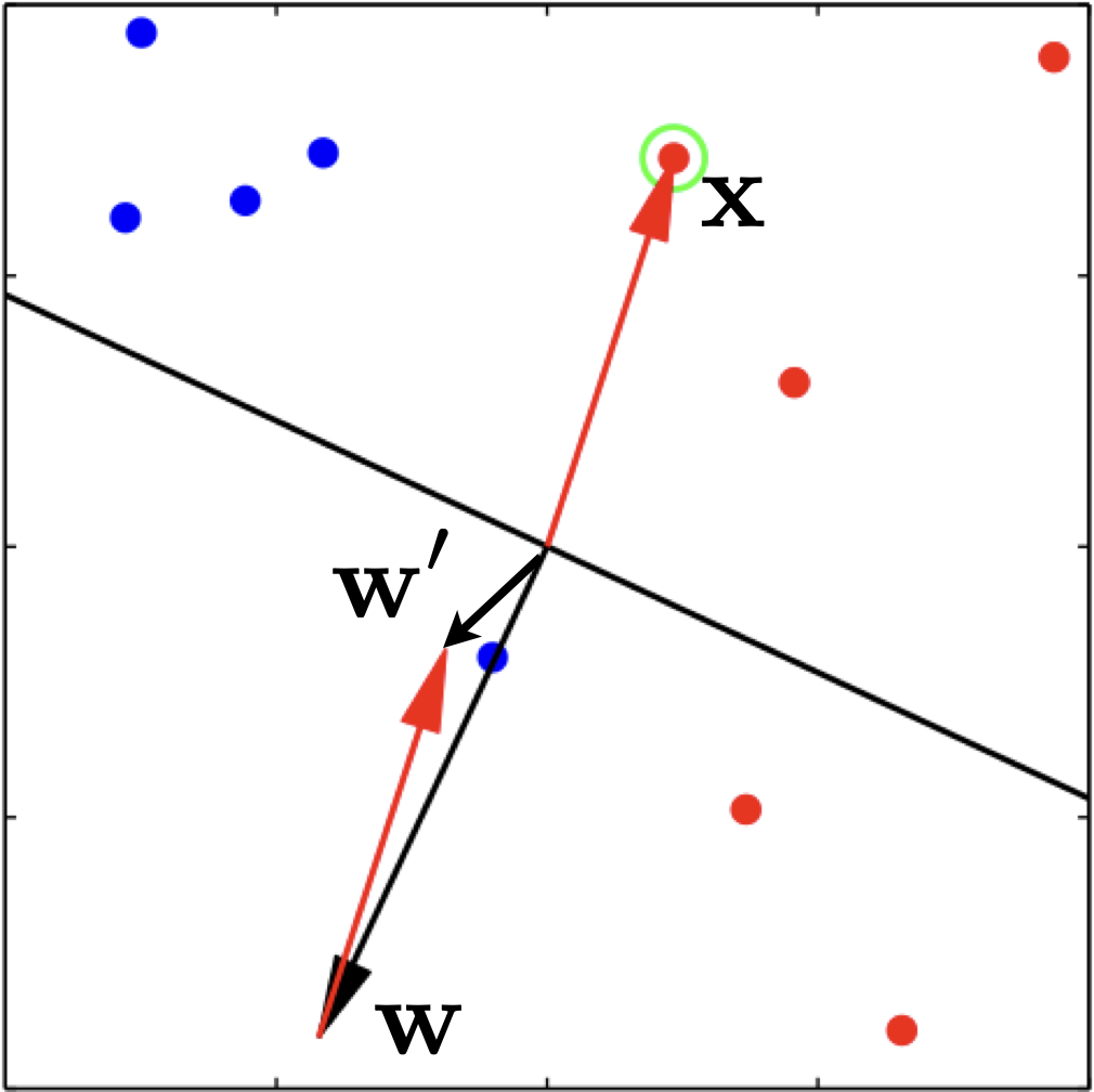
Here is an example update on a positive example.
Note, however, that after the update, we are not guaranteed to be correct on this example. The only thing we can be sure is that we will be less wrong on it. For example, in the above figure, example \(\mathbf{x}\) is positive (all green dots are positive), and the current weight vector \(\mathbf{w}\) points to the opposite direction which causes the dot product to be negative. After we apply the update, the new weight vector \(\mathbf{w}'\) is still wrong on this example, but much more aligned with it, i.e., much less wrong. In case in the next iteration over the training data, this example is incorrect again, we will apply another update, and eventually it will be correct.
Similarly, for a mistake on a negative example \(\mathbf{x}\) with \(y=-1\), we subtract \(\mathbf{x}\) from \(\mathbf{w}\):
\[ \mathbf{w}' \gets \mathbf{w} - \mathbf{x}\]
so that the new dot product is smaller (more negative or less positive).
We can unify the two update cases as:
\[ \mathbf{w}' \gets \mathbf{w} + y \cdot \mathbf{x}\]
We cycle through the whole training set multiple times, and if in one round, all examples are classified correctly by the weight vector (thus no update at all), we say the perceptron algorithm has converged.
However, it is not the case that perceptron can converge on all training sets. In practice, it does not converge on most data sets. In this case, when shall we terminate the training? Well, we can either set a predefined maximum number of iterations, or use the dev set to determine which round is the best round to prevent overfitting on the training set. Note that even when it can converge, it is likely to overfit on the training data, and even in that case we would prefer to use the dev set to stop the training before convergence.
The other important question is: how do we know if a training set will converge or not? That is the topic of the next exploartion.
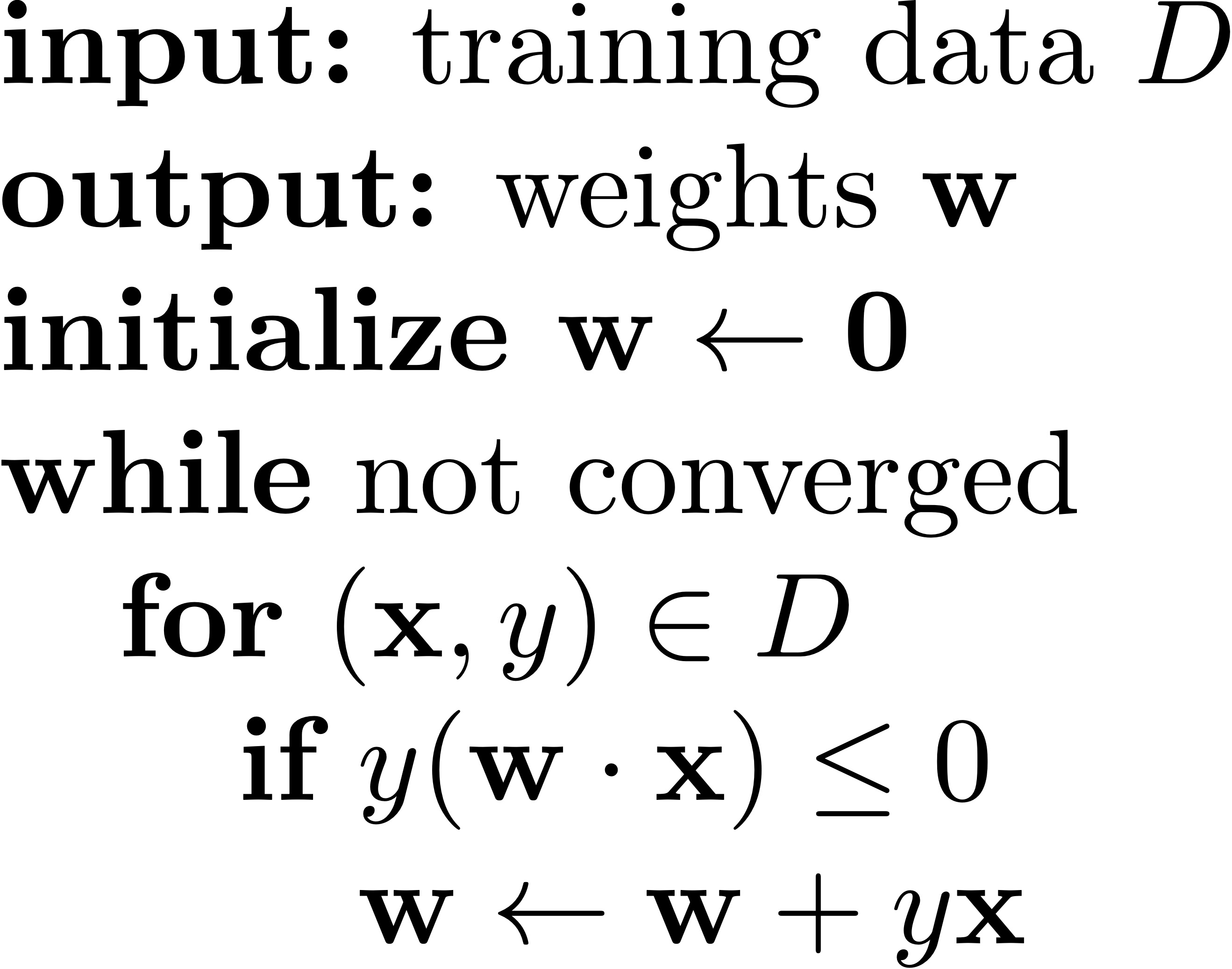
Now let us look at the pseudocode, which basically summarizes what we have discussed above.
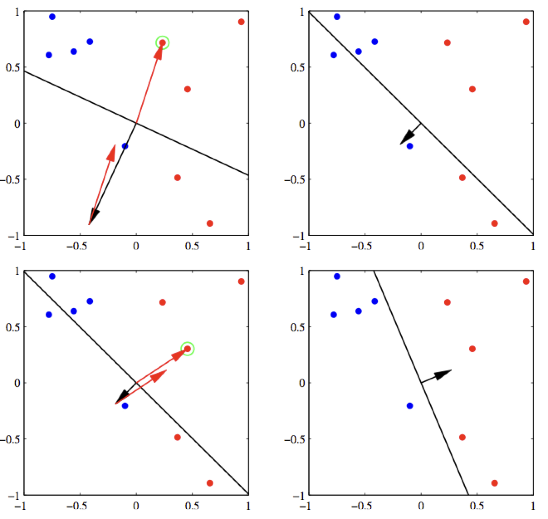
Here is a demo run of perceptron with two updates, and the final weight vector correctly classifies all examples.