In last section, we defined cost function \(J(\mathbf{w})\) to measure how good the linear model is with or without regularization. We want to find a weight \(\mathbf{w}\) to make the cost function as small as possible, which is an optimization problem. One common approach to optimization is iterative optimization, which generates a sequence of solutions in the attempt to reduce the objective (cost) functionto its smallest possible value. Formmally, if we want to optimize a function \(J(\mathbf{w})\) with variables \(\mathbf{x}\), i.e.,
\[\min_{\mathbf{w}}~J(\mathbf{w})\]
An iterative algorithm creates an sequence of solutions:
\[ \mathbf{w}^{(0)}, \mathbf{w}^{(1)}, ..., \mathbf{w}^{(k)}, ...\]
and hope for that \(J(\mathbf{w}) \rightarrow J(\mathbf{w}^\star) \rightarrow p^\star\) when \(k \rightarrow \infty\), where \(\mathbf{w}^\star\) is the optimial solution and \(p^\star\) is the optimial value of \(J(\mathbf{w})\).
One of the most popular iterative optimization algorithms for linear regression is Gradient Descent (also called Batched Gradient Descent in some context). The basic idea behind Gradient Descent is to iteratively update the model parameters (weights) by taking steps in the direction of the negative gradient of the cost function with respect to the weights. The negative gradient points in the direction of the steepest decrease of the cost function, which means that moving in that direction will result in a decrease in the cost function. To optimize \(J(\mathbf{w})\), the gradient descent algorithm starts with some initial \(\mathbf{w}\), and repeatedly perfroms the update:
\[ \mathbf{w}' \leftarrow \mathbf{w} - \alpha \frac{\partial}{\partial \mathbf{w}} J(\mathbf{w}) \]
Here, \(\alpha\) is called the learning rate. This is a very natural algorithm that repeatedly takes a step in the direction of steepest decrease of \(J\).
In order to implement this algorithm, we have to work out what is the partial derivative term on the right hand side. Let’s first work it out for the case of if we have only one training example \((\mathbf{x},y)\), so that we can neglect the sum in the definition of \(J(\mathbf{w})\) (without regularization). We have:
\[ \begin{aligned} \frac{\partial}{\partial \mathbf{w}} J(\mathbf{w}) & =\frac{\partial}{\partial \mathbf{w}} \frac{1}{2}\big(f_{\mathbf{w}}(\mathbf{x})-y\big)^2 \\ & =2 \cdot \frac{1}{2}\big(f_{\mathbf{w}}(\mathbf{x})-y\big) \cdot \frac{\partial}{\partial \mathbf{w}}\big(f_{\mathbf{w}}(\mathbf{x})-y\big) \\ & =\big(\mathbf{w}\cdot \mathbf{x}-y\big) \cdot \frac{\partial}{\partial \mathbf{w}}\big(\mathbf{w}\cdot \mathbf{x} - y\big) \\ & =\left(\mathbf{w}\cdot \mathbf{x}-y\right) \mathbf{x} \end{aligned} \]
For a single training example, this gives the update rule:
\[ \mathbf{w}' \leftarrow \mathbf{w} + \alpha (y - \mathbf{w}\cdot \mathbf{x})\mathbf{x} \]
The rule is called the LMS (least mean squares) update rule. This rule has several properties that seem natural and intuitive. For instance, the magnitude of the update is proportional to the error term \((y - \mathbf{w}\cdot \mathbf{x})\). As a result, if we are encountering a training example on which our prediction nearly matches the actual value of \(y^{(i)}\), then we find that there is little need to change the parameters; in contrast, a larger change to the parameters will be made if our prediction has a large error. Note that this update rule is very similar to the update rule for the perceptron algorithm in unit2.
\[ \mathbf{w}' \leftarrow \mathbf{w} + y\cdot\mathbf{x} \]
The main difference between the two update rules is that the perceptron algorithm updates the weight vector by adding the true label multiplied by the input vector, whereas the LMS algorithm updates the weight vector by adding the prediction error multiplied by the input vector.
We have derived the LMS rule for when there was only a single training example. When there are more than one example in a trainning set, we can sum up the gradient for each example, which is a natural extension.
\[ \frac{\partial}{\partial \mathbf{w}} J(\mathbf{w}) = \sum_{(\mathbf{x}, y)\in D} \left(\mathbf{w}\cdot \mathbf{x}-y\right) \mathbf{x} \]
To implement the gradient descent algrithm for linear regression, we just repeat the following update until convergence.
\[ \mathbf{w}' \leftarrow \mathbf{w} + \alpha \sum_{(\mathbf{x}, y)\in D} (y - \mathbf{w}\cdot \mathbf{x})\mathbf{x} \]
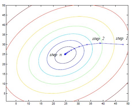
Note that gradient descent can be susceptible to local minima in general. However, the cost function \(J(\mathbf{w})\) is a convex quadratic function. As a result, the optimization for linear regression has only one global optima and gradient descent algorithm always converges (assuming the learning rate α is not too large) to the global minimum. The following figure illustrates the optimization process of gradient descent for a quadratic function. The figure below depicts the optimization process of gradient descent for a quadratic function, where the ellipses represent the contours of the quadratic function and the trajectory displays the parameter value at each step. We can observe from the optimization process that it will eventually reach the global minimum.
Notice that gradient descent algorithm needs to look at all examples at each step, which is correct but not efficient, especially when there are a lot of training examples. Instead, Stochastic Gradient Descent (SGD) is a variant of Gradient Descent that is commonly used for large-scale datasets. The basic idea behind SGD is to update the parameters after each training example, rather than after each epoch. This has the advantage of being much faster, since it doesn’t require us to scan the entire dataset before performing an update.
The update rule for SGD is similar to the gradient descent update rule, but instead of using the entire training set \(D\), we use a single randomly chosen training example \((\mathbf{x}^{(i)}, y^{(i)})\) at each iteration:
\[ \mathbf{w}' \leftarrow \mathbf{w} + \alpha (y^{(i)} - \mathbf{w}\cdot \mathbf{x}^{(i)})\mathbf{x}^{(i)} \]
Here, \((\mathbf{x}^{(i)}, y^{(i)})\) is a randomly chosen training example from \(D\). In practice, SGD is often more effective than vanilla gradient descent for large-scale datasets. This is because SGD updates the parameters more frequently, which can lead to faster convergence. However, SGD has a downside: the updates are noisy, since they are based on a single training example, and this can make the algorithm more difficult to converge.
Mini-Batch Gradient Descent is a compromise between batched gradient descent and SGD. Instead of using the entire training set or a single training example, mini-batch gradient descent uses a small batch of training examples at each iteration. This provides a balance between the stability of batch gradient descent and the efficiency of SGD.
The update rule for mini-batch gradient descent is similar to that of gradient descent and SGD, but instead of using the entire training set or a single training example, we use a batch of \(m\) randomly chosen training examples at each iteration:
\[ \mathbf{w}' \leftarrow \mathbf{w} + \alpha \sum_{(\mathbf{x}, y)\in D_m} (y - \mathbf{w}\cdot \mathbf{x})\mathbf{x} \]
Here, \(D_m\) is a subset containing \(m\) examples randomly chosen from \(D\), and \(m\) is the batch size.
In practice, mini-batch gradient descent is often the preferred optimization algorithm, as it provides a good balance between stability and efficiency. The choice of batch size is a hyperparameter that can have a significant impact on the performance of the algorithm. A larger batch size can provide a more accurate estimate of the gradient, but may also be more computationally expensive. A smaller batch size can be more efficient, but may result in a less accurate estimate of the gradient.
As is mentioned in last exploration, the cost function of linear regression often includes a regularization term. Indeed, the gradient descent algorithm can be applied to regularized linear regression as long as the regularized term is differentiable. For example, to minimize the cost function with \(\ell_2\) regularization, we can use a modified version of gradient descent called Ridge regression gradient descent. The update rule for Ridge regression gradient descent is:
\[ \mathbf{w}' \leftarrow \mathbf{w} + \alpha \sum_{(\mathbf{x}, y)\in D} (y - \mathbf{w}\cdot \mathbf{x})\mathbf{x} - \lambda \mathbf{w} \]
Note that the update rule includes an additional term that adds the derivative of the L2 regularization penalty term. This term serves to decrease the magnitude of the weights, which in turn reduces the chance of overfitting.