While linear regression is a powerful tool for modeling linear relationships, it has some limitations when it comes to modeling nonlinear relationships. Specifically, linear regression assumes that the relationship between the input variables and the output variable is linear, which means that it cannot capture nonlinear patterns in the data.
In Unit2, we have talked about the using nonlinear feature map to handle the inseparable cases for Perceptron. As a matter of fact, such technique can also be applied to linear regression to model nonlinear regression.
Recall that in our discussion about linear regression, we considered the problem of predicting the price of a house (denoted by \(y\)) from the size of the house (denoted by \(x\) instead of \(s\) in this exploration), and we fit a linear function of \(x\) to the training data. What if the price \(y\) can be more accurately represented as a nonlinear function of \(x\)? In this case, we need a more expressive family of models than linear models.
We start by considering fitting cubic functions \(y=w_3 x^3+w_2 x^2+w_1 x+w_0\). It turns out that we can view the cubic function as a linear function over the a different set of feature variables (defined below). Concretely, let the function \(\mathbf{\Phi}: \mathbb{R} \rightarrow \mathbb{R}^4\) be defined as
\[ \mathbf{\Phi}(x)=\left[\begin{array}{c} 1 \\ x \\ x^2 \\ x^3 \end{array}\right] \in \mathbb{R}^4 . \]
Let \(\mathbf{w}\) be the vector containing \(w_0, w_1, w_2, w_3\)as entries. We can rewrite the cubic function in \(x\) as
\[ y = \mathbf{w}\cdot \mathbf{\Phi}(x). \]
Thus, a cubic function of the variable \(x\) can be viewed as a linear function over the variables \(\mathbf{\Phi}(x)\). We will call \(\mathbf{\Phi}\) a feature map, which maps the raw feature \(x\) to the a set of new features.
Note that a feature map can be applied to more than one features. For example, We can consider two original features for house price prediction problem, house size \(x_1\) and number of bedrooms \(x_2\). Then we can use the following feature map to generate all the monomials of \(x\) with degree \(\leq 2\),
\[ \mathbf{\Phi}(\mathbf{x})=\left[\begin{array}{c} 1 \\ x_1 \\ x_2 \\ x_1x_2 \\ x_1^2 \\ x_2^2 \\ \end{array}\right] \in \mathbb{R}^6 . \]
Consider the following example dataset of 10 points:
| index | \(x\) | \(y\) |
|---|---|---|
| 0 | 0.1 | 0.658953 |
| 1 | 0.2 | 0.918608 |
| 2 | 0.3 | 0.850869 |
| 3 | 0.4 | 0.611410 |
| 4 | 0.5 | -0.010216 |
| 5 | 0.6 | -0.701915 |
| 6 | 0.7 | -0.685616 |
| 7 | 0.8 | -0.806996 |
| 8 | 0.9 | -0.577895 |
| 9 | 1.0 | -0.312153 |
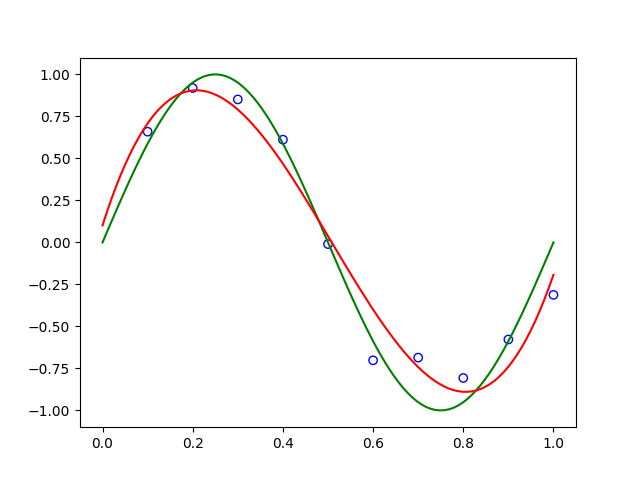
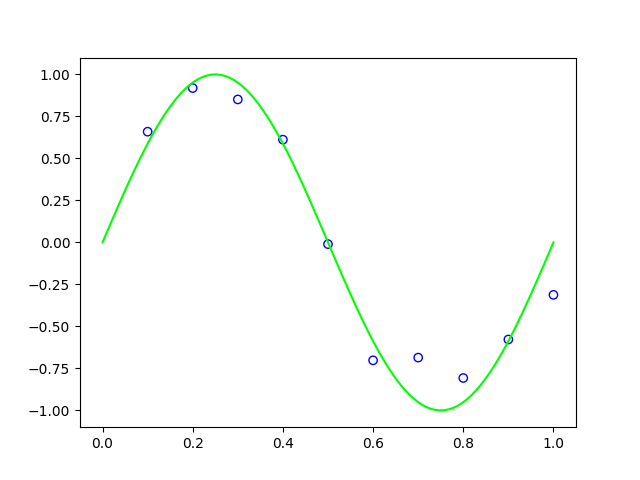
Those 10 data points are observed from the nonlinear relation \(y = \sin(2\pi x)\) in the domain \(0 < x \leq 1\). The scatters of the 10 points and the curve of the function \(y = \sin(2\pi x)\) are shown in the figure below.
Note that in reality, there is always some noise existing in observations. Therefore, the scattered points are usually not strictly on the curve. When we try to fit a straight line \(y = wx + b\), we get the following relation, \[ y = -1.9447x + 1.0641 \] which is shown as a red line in the following figure.
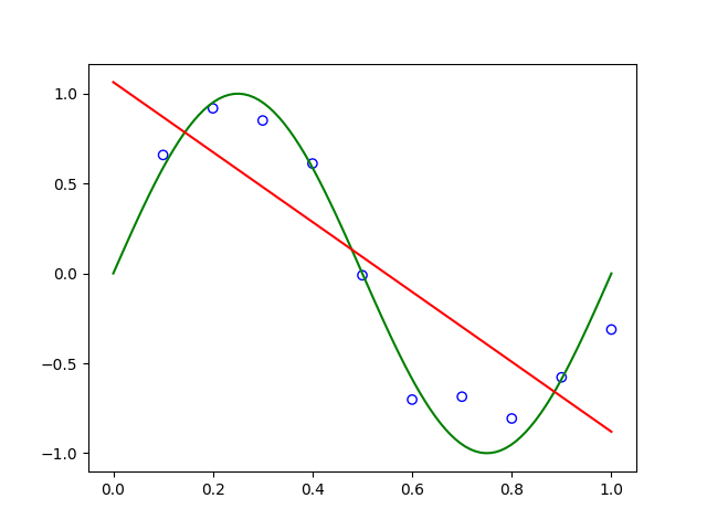
As we can see, the linear fitting is far away from the groud truth relation between \(y\) and \(x\). However, we can use the aforementioned cubic feature map to fit a cubic function \(y = w_0 + w_1x + w_2x^2 + w_3x^3\), and get a reuslt as
\[ y =0.1016 + 8.4591x + -25.5949x^2 + 16.8411x^3 \]
which is plotted in the figure below as a red curve. We can see the fitted curve is very close to our ground truth fucntion.