\(\renewcommand{\vec}[1]{\mathbf{#1}}\)
\(\newcommand{\vecw}{\vec{w}}\) \(\newcommand{\vecx}{\vec{x}}\) \(\newcommand{\vecy}{\vec{y}}\)
\(\newcommand{\sigmoidfnc}[1]{\frac{1}{1 + e^{-#1}}}\) \(\newcommand{\tanhfnc}[1]{\frac{e^x - e^{-x}}{e^x + e^{-#1}}}\) \(\newcommand{\relufnc}[1]{\max(0, #1)}\)
\(\newcommand{\norm}[1]{\lVert #1 \rVert}\) \(\newcommand{\normone}[1]{\norm{#1}_1}\) \(\newcommand{\normtwo}[1]{\norm{#1}_2}\)
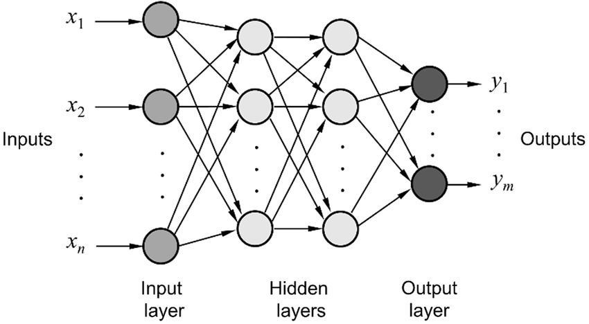
Multilayer Neural Networks, also known as Artificial Neural Networks (ANN) or Deep Neural Networks (DNN), are a powerful class of machine learning algorithms that can learn complex patterns and representations from the input data. It is a generalization of single-layer perceptron that we studied before. In this exploration, we will cover the basics of multilayer neural networks and how they are constructed.
A multilayer neural network consists of multiple layers of interconnected nodes or neurons. Each neuron computes a weighted sum of its input values and passes it through an activation function to produce an output value. The layers can be categorized into three types:
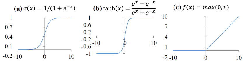
A neuron in a neural network computes a weighted sum of its input values and applies an activation function to produce an output value. The activation function introduces non-linearity into the network, allowing it to learn complex relationships in the data. Common activation functions include:
Forward propagation is the process of computing the output of a neural network given an input. The input values are passed through the network layer by layer, with each neuron computing its output value based on the weighted sum of its input values and applying the activation function. The output of the final layer is the output of the network.The forward propagation algorithm can be summarized as follows:
In order to train a neural network, we need to define a loss function that quantifies the difference between the predicted output and the true output. The objective of training is to minimize this loss function. Some common loss functions include:
Mean Squared Error (MSE) Loss: Used for regression tasks, this loss function calculates the squared difference between the predicted and true output values and averages it over all the examples. Mathematically, the MSE loss is defined as:
\[\ell(\vecy, \hat{\vecy}) = \frac{1}{N} \sum_{i=1}^N (y_i - \hat{y}_i)^2\]
where \(N\) is the number of examples, \(y_i\) is the true output, and \(\hat{y}_i\) is the predicted output.
Cross-Entropy Loss: Used for classification tasks, this loss function calculates the negative log-likelihood of the true class for each example and averages it over all the examples. Mathematically, the cross-entropy loss for a single example is defined as:
\[\ell(\vecy, \hat{\vecy}) = -\sum_{i=1}^C y_i \log(\hat{y}_i)\]
where \(C\) is the number of classes, \(y_i\) is the true class label (one-hot encoded), and \(\hat{y}_i\) is the predicted probability for class \(i\).
Backward propagation, also known as backpropagation, is an algorithm used to train multilayer neural networks. It involves computing the gradient of the loss function with respect to each weight by applying the chain rule. The gradient is then used to update the weights in the network to minimize the loss function. The backpropagation algorithm can be summarized as follows:
Training a multilayer neural network involves the following steps:
Overfitting occurs when a neural network learns the noise in the training data instead of the underlying patterns. This can lead to poor generalization to new, unseen data. Regularization techniques can be used to prevent overfitting. Common regularization methods include \(\ell_1\) and \(\ell_2\) regularization, dropout, and early stopping.
\(\ell_1\) and \(\ell_2\) Regularization: These techniques add a penalty term to the loss function based on the magnitude of the weights. \(\ell_1\) regularization adds the sum of the absolute values of the weights, while \(\ell_2\) regularization adds the sum of the squared values of the weights. This encourages the model to have smaller weights, making it less likely to overfit. Mathematically, the loss function with \(\ell_1\) or \(\ell_2\) regularization is defined as:
\(\ell_1\) Regularization: \[\ell_{\text{regularized}}(\vecy, \hat{\vecy}) = \ell(\vecy, \hat{\vecy}) + \lambda \normone{\vecw} \]
\(\ell_2\) Regularization: \[\ell_{\text{regularized}}(\vecy, \hat{\vecx}) = \ell(\vecy, \hat{\vecy}) + \lambda \normtwo{\vecw}\]
where \(\ell(\vecy, \hat{\vecy})\) is the original loss function \(\vecw\) is the weight of the model, and \(\lambda\) is the regularization parameter.
Dropout: Dropout is a regularization technique that involves randomly “dropping out” or setting to zero a fraction of the neurons in a layer during training. This prevents the model from relying too much on any single neuron and encourages the model to learn more robust representations. Dropout is applied only during training, and during inference, all neurons are used with their weights scaled by the dropout rate.
Early Stopping: Early stopping involves monitoring the performance of the model on a validation set during training and stopping the training process when the performance on the validation set starts to degrade, indicating that the model is starting to overfit. This technique helps to find the optimal point in training where the model has the best generalization performance.
By applying one or a combination of these regularization techniques, overfitting can be mitigated, leading to better generalization of the neural network to new, unseen data.