\(\renewcommand{\vec}[1]{\mathbf{#1}}\)

\(\newcommand{\vecv}{\vec{v}}\) \(\newcommand{\vectheta}{\pmb{\theta}}\)

Exploration 4.2: NLP Case Study: Word Embeddings

Word embeddings are continuous vector representations of words that capture semantic and syntactic relationships between words. They have been shown to significantly improve the performance of many natural language processing (NLP) tasks. In this exploration, we will cover the basics of word embeddings, their properties, and how they can be trained.

From One-Hot to Continuous Representation

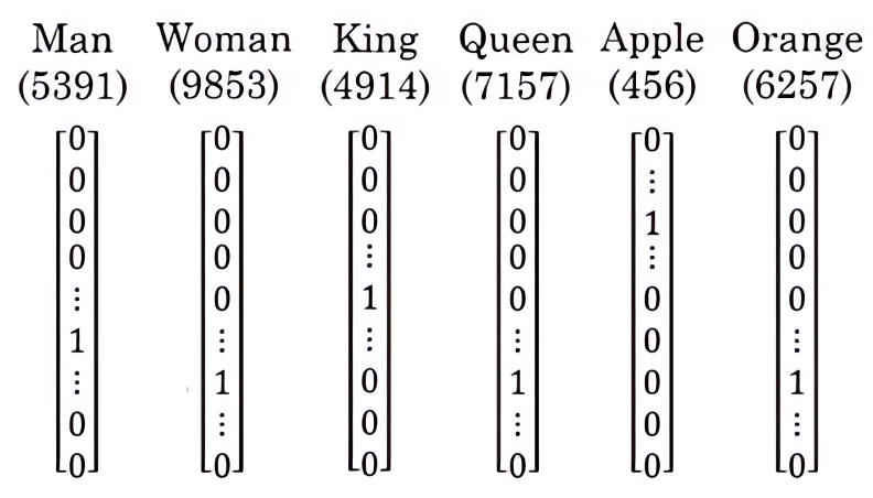
Traditionally, words were represented using one-hot vectors, where each word in the vocabulary is assigned a unique index (e.g., in the following example, “Orange” is assigned the index of 6257) and is represented as a binary vector with a single 1 in the position corresponding to the word’s index and 0s elsewhere. To convert a word to its one-hot vector representation, a look-up process is employed: first, the word’s index is determined from the predefined vocabulary, and then a vector of the same length as the vocabulary is created, with the element at the word’s index set to 1, and all other elements set to 0.

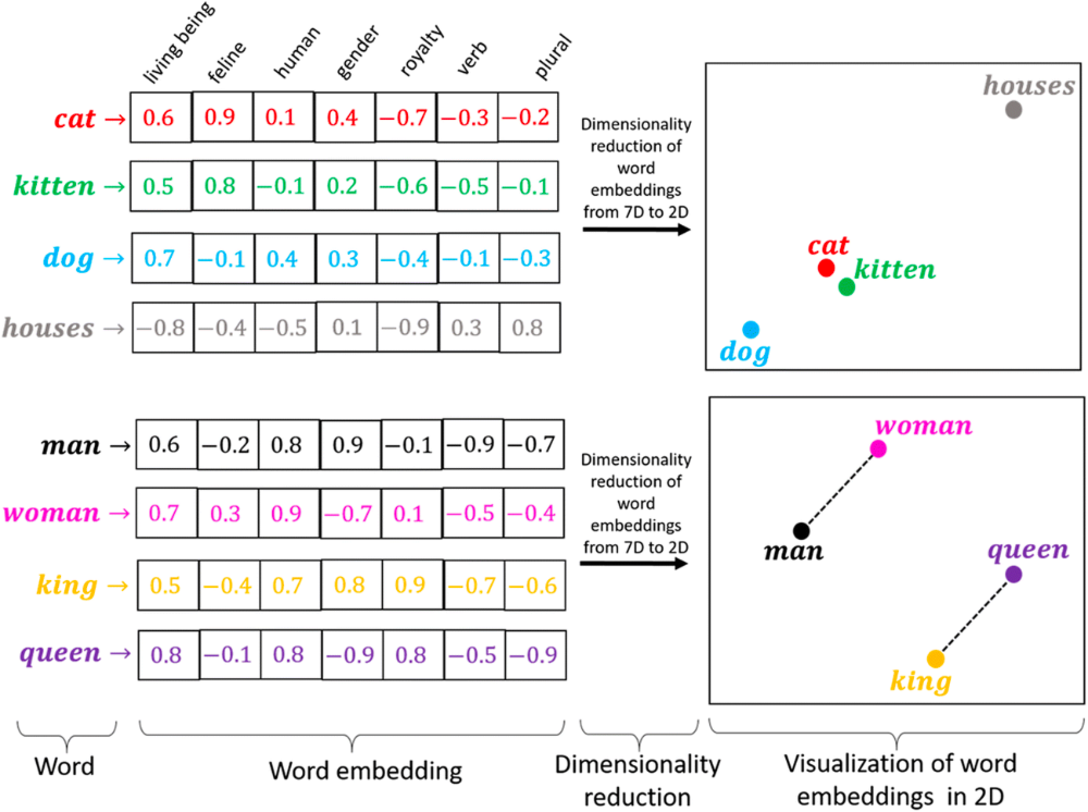
However, one-hot representations are sparse and do not capture any semantic information about the words. To address this limitation, continuous representations such as word embeddings are used. These dense vector representations are capable of capturing semantic and syntactic relationships between words, making them more suitable for NLP tasks.

Properties of Word Embeddings

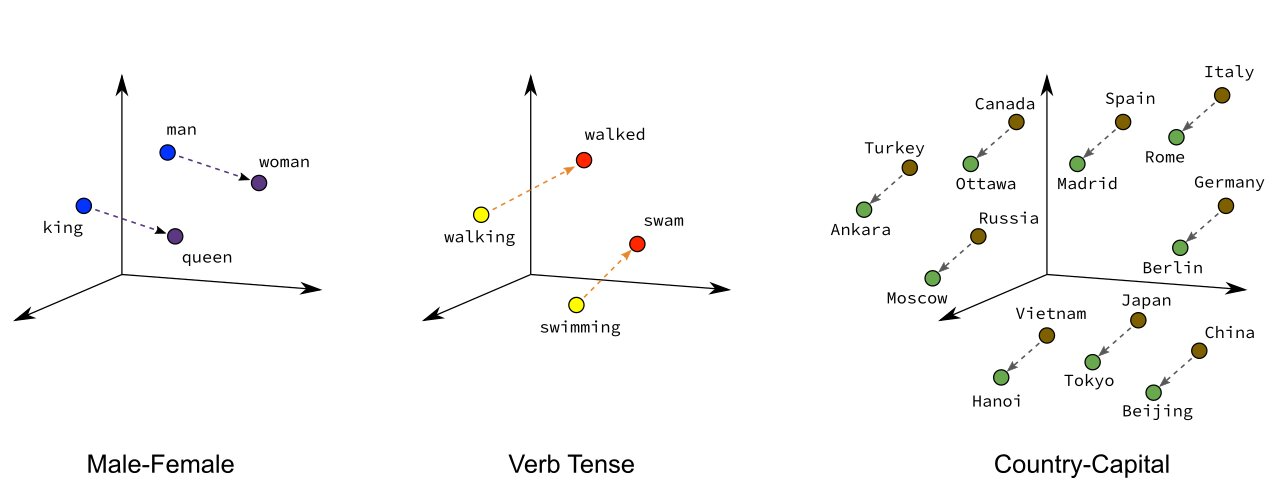
Some interesting properties of word embeddings include:

1. Similar words have similar embeddings: The embeddings of semantically similar words tend to be close together in the vector space. This can be measured using cosine similarity, which computes the cosine of the angle between two vectors. For example, the cosine similarity between the embeddings of the words “cat” and “kitten” would be higher than the cosine similarity between “cat” and “tree”.

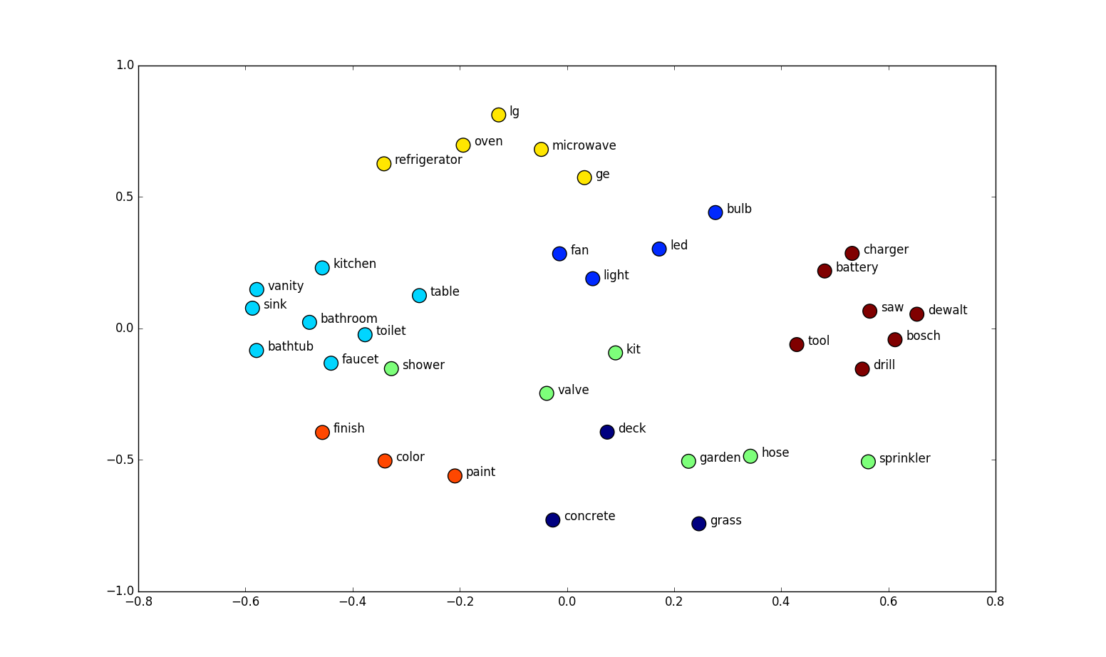
2. Analogies: Word embeddings can capture analogies, such as “man - woman = king - queen”. This can be illustrated by performing vector arithmetic on the embeddings and finding the closest word in the vector space. For example:

   \[\text{embedding}(\text{"man"}) - \text{embedding}(\text{"woman"}) + \text{embedding}(\text{"queen"}) \approx \text{embedding}(\text{"king"})\]

3. Visualizations: Word embeddings can be projected to a lower-dimensional space (e.g., using t-SNE or PCA) for visualization purposes. This can help in understanding the relationships between words and identifying clusters of similar words.

Model and Training

There are several models and algorithms for learning word embeddings, including:

1. Word2Vec: A family of models (Skip-gram and Continuous Bag of Words) that learn word embeddings using a shallow neural network. Word2Vec is trained to predict a word given its context (Skip-gram) or the context given a word (Continuous Bag of Words).

   1. In the Word2Vec model, a corpus is represented as a sequence of words, \(w_1, w_2, ..., w_n\), where each \(w_i\) corresponds to the \(i\)-th word in the corpus, and \(n\) is the total number of words in the corpus. The indices in the one-hot encoding representation corresponding to each word are used for training the model.

   2. Skip-gram: The Skip-gram model is trained to predict the context words given a target word. For example, given the sentence “The cat is on the mat”, the model would be trained to predict the words “The”, “cat”, “on”, and “the” when given the word “is”. The context window size determines how many words before and after the target word are considered as context. The objective function for the Skip-gram model is as follows: \[J(\vectheta) = \frac{1}{n}\sum_{t=1}^{n}\sum_{-m\leq j \leq m, j \neq 0} \log p(w_{t+j} \mid w_t; \vectheta)\] where \(n\) is the total number of words in the corpus, \(w_t\) is the target word, \(w_{t+j}\) is a context word, \(m\) is the window size, and \(\vectheta\) represents the model parameters. The probability \(p(w_{t+j} \mid w_t; \vectheta)\) is usually modeled using the softmax function: \[p(w_{t+j} \mid w_t; \vectheta) = \frac{\exp(\vecv_{w_{t+j}} \cdot \vecv_{w_t})}{\sum_{w'=1}^W \exp(\vecv_{w'} \cdot \vecv_{w_t})}\] where \(\vecv_{w}\) is the input vector for word \(w\), \(\vecv_{w'}\) is the output vector for word \(w'\), and \(W\) is the vocabulary size.

   3. Continuous Bag of Words (CBOW): The CBOW model is trained to predict the target word given its context words. For example, given the same sentence “The cat is on the mat”, the model would be trained to predict the word “is” when given the words “The”, “cat”, “on”, and “the”. Similar to the Skip-gram model, the context window size determines how many words before and after the target word are considered as context. The objective function for the CBOW model is: \[J(\vectheta) = \frac{1}{n}\sum_{t=1}^{n} \log p(w_t \mid w_{t-m}, ..., w_{t-1}, w_{t+1}, ..., w_{t+m}; \vectheta)\] The probability \(p(w_t \mid w_{t-m}, ..., w_{t-1}, w_{t+1}, ..., w_{t+m}; \vectheta)\) is modeled using the softmax function: \[p(w_t \mid w_{t-m}, ..., w_{t-1}, w_{t+1}, ..., w_{t+m}; \vectheta) = \frac{\exp(\vecv_{w_t} \cdot \overline{\vecv}_c)}{\sum_{w'=1}^W \exp(\vecv_{w'} \cdot \overline{\vecv}_c)}\] where \(\overline{\vecv}_c = \frac{1}{2m} \sum_{-m\leq j \leq m, j \neq 0} \vecv_{w_{t+j}}\) is the average of the input vectors for the context words.

   4. Both the Skip-gram and CBOW models learn to represent words as dense vectors in a way that captures their semantic and syntactic relationships, which makes them useful for a variety of NLP tasks.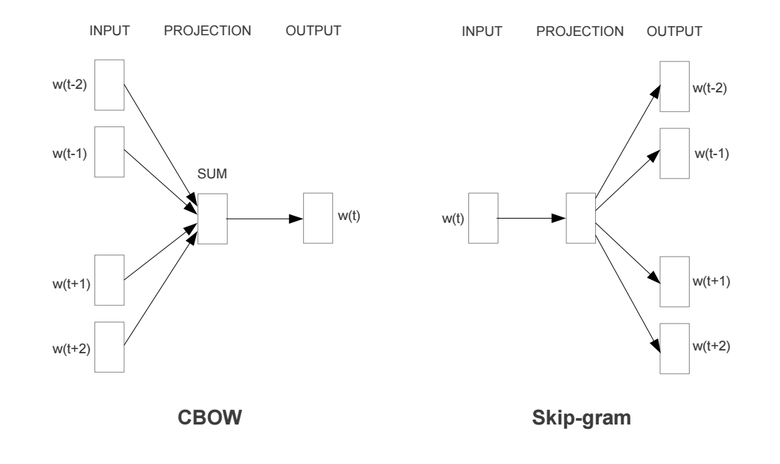

2. GloVe (Global Vectors for Word Representation): A model that learns word embeddings by factorizing a word co-occurrence matrix. The main idea behind GloVe is that the relationships between words can be encoded in the ratio of their co-occurrence probabilities. GloVe is trained to minimize the difference between the dot product of word vectors and the logarithm of their co-occurrence probabilities. By doing so, it learns dense vector representations that capture semantic and syntactic information about words.

3. FastText: An extension of the Word2Vec model that represents words as the sum of their character n-grams. FastText can learn embeddings for out-of-vocabulary words and is more robust to spelling mistakes. FastText can be trained using either the Skip-gram or CBOW architecture, similar to Word2Vec.

To train word embeddings, a large text corpus is required. The text corpus is preprocessed (e.g., tokenization, lowercasing) and fed into the chosen model. The model learns the embeddings by updating its weights using gradient-based optimization algorithms (e.g., stochastic gradient descent).

Pretrained Word Embeddings

In many cases, it is not necessary to train word embeddings from scratch. There are several pre-trained word embeddings available that can be used directly in NLP tasks or fine-tuned for specific domains. Some popular pre-trained word embeddings include:

1. Google’s Word2Vec: Pre-trained on the Google News dataset, containing 100 billion words and resulting in a 300-dimensional vector for 3 million words and phrases.

2. Stanford’s GloVe: Pre-trained on the Common Crawl dataset, containing 840 billion words and resulting in 300-dimensional vectors for 2.2 million words.

3. Facebook’s FastText: Pre-trained on Wikipedia, containing 16 billion words and resulting in 300-dimensional vectors for 1 million words.

I have added more details on the properties of word embeddings, including some examples, and explained how to use pretrained embeddings in NLP tasks in the word_embeddings.md file below:

Using Pretrained Word Embeddings in NLP Tasks

Pretrained word embeddings can be used as a starting point for various NLP tasks, such as text classification, sentiment analysis, and machine translation. They can be used in the following ways:

1. As input features: The word embeddings can be used as input features for machine learning models, such as neural networks or support vector machines. For example, in a text classification task, you could average the embeddings of all words in a document to obtain a document-level embedding, which can then be used as input to a classifier.

2. As initialization for fine-tuning: In some cases, it might be beneficial to fine-tune the pretrained embeddings on a specific task or domain. You can initialize the embedding layer of a neural network with the pretrained embeddings and then update the embeddings during training. This can help the model to better capture domain-specific knowledge.

3. In combination with other embeddings: Pretrained embeddings can be combined with other types of embeddings, such as character-level embeddings or part-of-speech embeddings, to create richer representations for NLP tasks.

By using pretrained embeddings, you can leverage the knowledge captured from large-scale text corpora and improve the performance of your NLP models.

Contextualized Word Embeddings

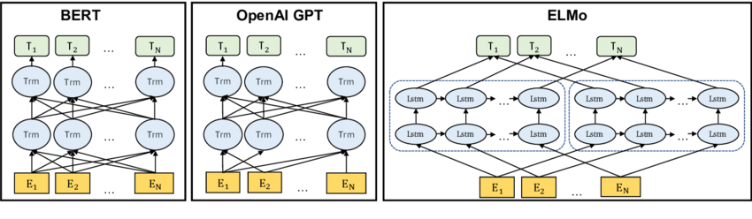
Traditional word embeddings, like Word2Vec, GloVe, and FastText, assign a single vector representation to each word. However, this static representation may not be sufficient to capture the different meanings of a word in different contexts. Contextualized word embeddings, such as ELMo, BERT, and GPT, address this limitation by generating dynamic word representations that depend on the context in which the word appears. These models are trained on large-scale language modeling tasks and have been shown to further improve the performance of NLP tasks.

Videos

• one-hot vectors
• word embeddings
• contextualized word embeddings